An Object-Oriented Simulation of a Reactive Manufacturing Scheduling System
Molu Olumolade
Industrial and Engineering Technology Dept.
Central Michigan University
Mt. Pleasant, MI 48859
Olumo1mo@cmich.edu
Abstract
An object-oriented simulation model was developed for testing and evaluating an intelligent manufacturing scheduling system. The object-oriented paradigm facilitates the emulation of real-life data and enhances modularization and integration of the system. The object-oriented simulation architecture includes a database which stores simulation-related data without changing its structure. The model uses both standard and modified dispatching rules under an overall system objective of minimizing total due date penalties. The simulation is used to select configuration elements and execute replication runs during testing and for evaluation. Output data on cell and machine loading and performance are presented concurrently in graphical form during simulation.
Introduction
Manufacturing systems have become more difficult to analyze using traditional analytical methods such as linear or nonlinear programming, queuing network or queuing theory due to the development of new technologies such as Flexible Manufacturing Systems (FMS). Simulation has emerged as a viable approach for assessing the capabilities and performance of these newer flexible systems under a variety of conditions.
The standard procedure for manufacturing system simulation has been to design and construct the model, validate and verify the simulation, and then to run the simulation and analyze the results. Various "what-if" scenarios can be selected based on these results and used in a repeat of this process.
There are many methodologies (direct experiment, analytical procedures, numerical analysis and simulation modeling) that are available for the design, analysis and evaluation of manufacturing systems. Among these, simulation has been criticized on the basis that:
· Statistical inferences from its results are subject to statistical errors that are not controllable;
· There are approximation errors in numerical solutions;
· Considerable time and effort can be required for information gathering, modeling and programming.
Nonetheless, simulation is still the most adaptable and convenient approach for detailed analysis and evaluation of manufacturing systems both at the design and implementation stage. Simulation can include on a real-time basis such operational factors as uncertainty in arrival rates, operation times, and machine availability and can represent the manufacturing system to any desired level of detail. Modern simulation is usually discrete-event based, and the modeling environment is increasingly object-oriented. The use of an object-oriented architecture can reduce development time, as well as the time and cost of subsequent changes.
This paper describes a simulation system developed to test and evaluate a manufacturing scheduling system. The object-oriented paradigm adopted facilitates emulation of real-life data for use in the simulation system and enhances modularization and integration of the system.
Relevant Research on FMS Modeling
Numerous models have been developed for analyzing the performance of FMS. In general, these models cannot be used as generative or prescriptive tools for optimizing system performance under specific conditions and criteria, although some have been used to generate guidelines for optimal operation and control of the system. In a recent comparison of scheduling rules Kurz and Askin12 found that no one rule satisfies all situations.
Donath and Graves7 introduced a mathematical model makespan for flexible assembly systems that minimizes the makespan. The system is viewed as a collection of flexible workplaces for both manual and automated assembly. Melouk et al.18 also minimized makespan for a single batch-processing machine using simulated annealing. Simulation and expert system (knowledge‑based) approaches are also used for solving FMSs problems. Feuer, et al.8 discussed a real life simulation‑based scheduling system which considered multiple performance measures (low work-in‑process, high machine utilization and short lead times). Driving shop floor in real time was the goal of Son et al.23, using a multipass scheduling algorithm.
Mean flow time, number of tardy jobs, and the number of tool changes are used in assignment rules by Melnyk, et al.17 for simulation of tooling constraints and shop floor scheduling in a system operating under varying levels of tooling availability. The simulated shop is broken into two components. The first consists of a single‑machine work center, which is modeled, in detail. The second represents the remainder of the shop in aggregate which is added to provide competition for the tools in the work center.
Bispo and Sentierio1 present an algorithm using a schedule space search characterized by a heuristic-oriented approach based on simulation. The algorithm can be considered as a look-ahead dispatching rule, since the simulation-based search forecasts how good a schedule can be before the best one is chosen. A genetic algorithm was employed by Keung et al.11 to solve the problem of multiple machines tool selection and by Chryssolouris and Subramaniam5 to address mean job tardiness and cost.
Chen et al.4 considered an optimization-based approach to maximize on-time delivery of products, reduce inventory and the number of setups. Mandelbaum and Hlynka16 explored the benefits of using an expert’s estimate of unknown service times to order a batch of jobs of fixed size prior to machine processing. In order to reduce the weighted number of late deliveries for a single machine, Phojanamongkolkij et al.20 used a weighted forward algorithm. Denton and Gupta6 increased the utilization of resources with a bounding approach whose upper limits are independent of job duration distribution.
There has been considerable exploration of the object-oriented paradigm for the simulation of manufacturing systems Thomasma et al.24, Boukachour2, and Zobel and Cummings27. Other paradigms such as access-oriented and logic-oriented have also been considered, but none has the same impact on program reusability as the object-oriented paradigm. Recently, to enhance the use of object-oriented systems, Hardgrave and Johnson9 used the theory of planned behavior, goal-setting theory and technology acceptance model (TAM) to develop a model to explain the acceptance of object-oriented system development.
Other recent contributions include Zhang et al.26, Laporte et al.14, Morton and Popola19, and Jans and Degrave10.
In the system presented in this paper, the object-oriented architecture includes a database that stores simulation-related data without changing its structure. The simulation was used to select and carry out the desired replication runs of the reactive scheduling system under a range of testing conditions. Output on cell and machine loading and performance is presented concurrently in a graphical form during the simulation
Description of the Cellular Manufacturing System (CMS)
The cellular manufacturing system configuration used for testing in this simulation consists of two different cells each containing between four to six workstations (machines or inspection workstations). Each cell has material and tool storage that are accessible from all machines in the cell.
To maximize space utilization, each cell rather than each workstation (i.e. machine) is equipped with central buffers, one for arriving jobs and one for work-in-process (WIP). All of the completed parts in a given job are assumed to be immediately removed to the finished goods storage area. Each job consists of a batch of parts with its specification of quantity, due date, date ordered and due date tolerance as defined by the consumer. Due date tolerance is negotiated between the consumer and the manufacturer. It specifies a time frame within which a job cannot be penalized if completed. Any job completed outside this time frame will incur either an early or late penalty. Each job also has a secondary due date; beyond which the job even if completed will not be accepted by the customer.
Each job has no specific order for leaving the cell once it enters, since a job that enters first may not necessarily be the first to be completed. For example, the job with the shortest processing time would be expected to leave the cell first when using the shortest processing time dispatching rule and one with the earliest due date when the earliest due date dispatching rule is employed.
Description of Simulation Input Data
It is not always possible to use actual production input data in a simulation, and in fact, this is not always necessary even when it is possible. An alternative to actual data is “pseudo-data" generated from a standard distribution. When data is synthesized in this way, the parameters of the distribution are chosen to reflect the properties of the real system. For simulation testing in the present research, pseudo-data generated from standard distributions are used where necessary. The key input data include Process Plan, Demand Data, Material Data, Tool data, Machine data, and Machine Failure.
Establishing the Modeling Criteria
In a simulation, the objectives or goals of the system being tested have to be defined. These objectives need to be prioritized in order of importance. In this model, the following objectives are considered:
· Operating within the limits of the system
· Meeting demand due dates
· Minimizing material and work-in-process inventory
· Minimizing the total delinquencies (total earlobes and tardiness)
In the present case, the most important objective is the meeting of demand due dates. This requires minimization of the total earliness and lateness of all jobs that are delinquent of this goal. To meet the above objective, the following scheduling rules were utilized.
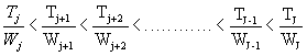
Earliest Due Dates (EDD): EDD is the first rule to be considered in sequencing jobs through the system. Initially, all jobs waiting to be scheduled are sequenced in an ascending order of their due dates between cells. That is, dj < dj+1 < dj+2 < . . . . . . . . . . < dJ-1 < dJ. As new jobs continue to arrive into the system, the rule reverts to the modified due date that determines the correct order of processing. Modified due dates calculate the time remaining to due date on each job (Mdj = dj – ėj) where
Mdj = modified due date of job j
dj = the due date of job j
ėj = expired time to the point of decision, which is current date minus arrival date (cj – aj).
From this point jobs are sequenced in the order of Mdj < Mdj+1 < Mdj+2 < . . . . . . . MdJ-1 < MdJ
Weighted Shortest Processing Time (WSPT): This rule is operational only if after instituting the two rules above, there are ties among jobs. In this case each job is assigned a weight (wj) that is based on the importance of the job; this importance may be related to customer contribution to a company’s annual revenue. This rule is designed to minimize flowtime of all jobs (j Є J) within a given cell, and it is defined as:
 where Tj
= the total processing time of job j and Wj
= the weight of job j the jobs are henceforth sequenced in the ascending order
of WSPT, where
where Tj
= the total processing time of job j and Wj
= the weight of job j the jobs are henceforth sequenced in the ascending order
of WSPT, where
Shortest Operation Processing Times (SOPT): In SOPT, each operation of parts in a job is considered individually and are arranged in an ascending order of their processing times; tij is the processing time of operation i on job j (i = 1, 2, . . . . . . . I). SOPT arranges parts such that time for operation 1 of part p in job j (t1pj) is less than processing time of operation 2 (t2pj) on the same part. (tipj < t(i+1) pj< t(I+2)pj < . <t(I-1)pj < tIpj). The rule is used to assign operations to an individual machine for processing.
Object-Oriented Design Architecture
The object-oriented methodology used was structured analysis, which is a top-down procedure using a hierarchical data flow process to describe and analyze each lower level process. For the simulation system, the initial steps involve the description of the manufacturing system in terms of objects and the definition of appropriate tools for models and their simulation. The following description of the modules should be read in conjunction with Figure 1:
The user interface module allows input of the manufacturing system and the scheduling requirements. The user can define and input the hierarchical levels of the resources, the structural descriptions of the different operations (process plan, demand, etc.), and their attributes.
1. Appropriately, external entities such as customer demand can also be described. Each individual element and data, which has been specified, is stored in a data dictionary.
2. The Structural Description Level module contains the description of the structural language. This is the context preparation block, which defines the interconnections between all of the different operations.
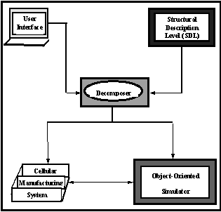 |
Figure 1: Object Oriented Structure
3. The Translator or Decomposer Block translates and decomposes all of the information from the previous modules and generates data usable in the simulation module.
4. The Cellular Manufacturing System (CMS) module describes the configuration of the manufacturing physical entities (resources), their locations (cells), capacities, and their interrelationship with other entities outside the same cell or environment. It also includes the management and system objectives.
5. The Simulator module is a discrete event-driven simulator. This is an important module that integrates the functional entities of the manufacturing system. The integration allows real-world data utilization. It also serves as a diagnostic and evaluative tool for the system. The results and the control information from this module are shared with the manufacturing system module. In the Simulator module, there are objects which define the message flow structure for the interaction among models, the physical and high level entities, the statistical phase and so on. The Simulator verifies the correctness of the scheduling system in terms of optimality, feasibility, and satisfaction of the criteria described in the CMS module.
6. The Scheduling modules are the most important modules in the system. They specify the dispatching rules with the necessary algorithms needed to satisfy management and system objectives. Both the Simulator and the manufacturing system use the scheduling function of these modules. The diagnostic tool incorporated gives the system status at any given stage. It reveals when a machine breakdown occurs, when a machine is overloaded, or when the entire system can absorb an incoming job. It interacts with both the Simulator and the Scheduling modules. Most management decisions during real-world operation are based on the results from the diagnostic tool.
7. The Model Acceptance module (outside of but operating in conjunction with the Simulator) evaluates the solution obtained against management and system objectives and decides whether the result is acceptable or not. If it is acceptable, the module stores the information; otherwise, further modification is carried out through the system improvement procedure built inside the scheduling module. This process continues until an acceptable schedule is obtained or until external changes are made which allow satisfaction of the system objectives. It should be emphasized that most changes made in order to satisfy system objectives are preferable in the scheduling module rather than in the simulator.
Design Philosophy and Strategy
The modeling environment is very important in any simulation system; it determines the type of information in existence in the system. The model layout (Figure 2) defines the relationship between the physical elements and algorithmic procedures and statistical parameters. Figure 3 shows the simulation design architecture. The stochastic parameters include the statistical distribution and uncertainties in information, variations in shop floor activities (such as changes in demand), machine failure, and variations in machine workload and utilization.
The first activities in any simulation experiment are defining the problem and establishing the objectives of the experiment. The system borders must be drawn and the key real objects specified or identified. These objects are either resources in the layout or products. In carrying out the experiment, the following are the major sub-tasks:
Determine the job flow between workstations and between cells.
· Determine the flow constraints.
· Invoke the scheduling system using all of the pre-described modules.
· Analyze the results from the scheduling system.
· Select the most feasible and optimal schedule from among the many alternatives.
|
|
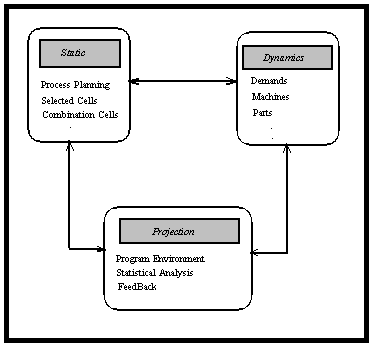
Figure 2 Simulation Model Elements
The simulation system can be viewed as both an object representation for facility and product information and as an architecture and testbed, which combines many of the elements of the scheduling system. It can also be considered as a process as well as an event-oriented modeler. In the manufacturing context, a process-oriented model can be defined as one that follows the sequences parts operations. A process-oriented model can with no loss of application be transformed into an event model, since a process is not only a sequence of operations but also a sequence of events.
Object-Oriented Implementation
The implementation of the system as an object-oriented environment has numerous advantages. A major characteristic of the object-oriented paradigm is its modularization mechanisms which allow each entity to be represented as an individual object. In order to achieve execution and modification efficiency, object level modularization requires that information relating to an object should be contained in the object and that a class object consists of a collection of such objects. In the object-oriented paradigm, the abstraction of concepts is easily achieved by using class definitions and instantiation of the objects. Hierarchical abstraction can be achieved through the use of the property of class inheritance. An advantage of an object-oriented system is that it provides a graphical, interactive programming environment in which the user's world can be modeled in terms of objects and messages. The power of object-oriented programming itself lies in two conceptual foundations: encapsulation and inheritance. Encapsulation provides protection of objects from unauthorized changes by restricting access to the objects. Inheritance describes the enhancement of new specialized sub-classes, which inherit the data, and behavior of higher-level generic super classes.
Grouping
of the System Elements
One of the characteristics of the object-oriented paradigm
is its enhancement of modularity of programming structures.
The model elements (shown in Figure 2) can be grouped under the three
headings of static, dynamic, and projection elements.
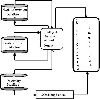
Figure 3:
Object-Oriented Stimulation Architecture
i) Static Elements
Static elements are those which, despite the random effect of the system environment, remain invariant during the entire execution phase. This group includes the initial process plan which remains constant during the process. Also included are the cells selected for a part, according to the process plan or alternate process plan (APP). If the cell selection arriving from the basic process plan is no longer valid (because of e.g. machine breakdown), the alternate process plan (APP) can be used to select a substitute cell for a part operation.
ii) Dynamic Elements
The dynamic elements describe the different states of the system at given times. According to the compatibility rule, these elements are descendants of the static elements. Dynamic elements in the system include such variables as the state of a machine, parts, demands, raw materials and tools. The simulation system monitors the actions of these elements and collects statistical results on each. In the present system, a dynamic element was represented through a production rule hard-coded in the object-oriented environment. For example, if a system element is in a certain state, it has to satisfy certain constraints before exiting that state. One such constraint when a machine fails is:
MAIT >= MTTR
ifTrue:[ No action Necessary]
ifFalse: [ Remove Affected parts & Return to SIMP].
MAIT is the maximum allowable idle time. It defines the maximum time a machine can be idle and still be able to complete its assignment. MTTR is the mean time to repair the failed machine. When the system signals a machine failure, the MTTR is immediately generated (or could be input from the user, should empirical data be available). The obtained value is compared with MAIT to determine the next cause of action to take.
iii) Projection Elements
Projection elements describe the way in which the application is presented to the user. In this model, presentation takes two forms: the first is the execution mode presentation, which is depicted graphically. The other is the final result, which is presented in textual form. Both are represented in a simple and explicit manner such that the user interacts with and feels comfortable within the environment.
Object Modeling
The use of an object-oriented approach to create the model for this system derives naturally from the fact that every physical system consists of objects and their interactions. These objects are structured hierarchically in classes. Each class has attributes that account for the characteristics and procedures which define its behavior. At the top of each hierarchy is the class object, identified by the object type. Each of the four major actors (class objects) in the system has an object type slot and instances attached to it.
All objects in the system are grouped into object classes. Individual objects of the same type belonging to a class are instances of that class. Instances of the same class share the properties of the class. Objects are characterized by attributes, and attributes are specified by values. While the attributes of an object do not change, values do due to the dynamic nature of the environment. For example, a machine could be classified as machine object, and one of its attributes could be an allocation index or assigned workload. Naturally, the values of this attribute undergo continuous changes, and hence proper procedures should be defined to obtain proper and accurate values of the attribute at each stage of the simulation.
Messages
Messages are the (only) means by which objects communicate with each other. A message may have one or more arguments. A message received by an object triggers the execution of a procedure (method) to produce the required behavior. Any object receiving a legitimate message then takes some action, processing the message internally and/or sending a message to other objects. During the development of the scheduling system, these questions arose:
§ how should these messages be presented in order to maintain adequate understanding and resolve conflict of interpretation among objects.
In the system, the only elements actually performing actions (or causing an action to be performed such as retrieving a record from a file, determining the value of a variable, etc.) are the process elements. Therefore, it is reasonable that only these objects be allowed to send messages to other objects. These messages should not appear on a traditional data flow structure. A data flow is here considered as either an input into the process or internally generated data. A data flow will often involve the argument of a message sent from a process object to another object. However, an element of data as shown and stored in a data dictionary is just that: a data element.
Methods
A method is another name for a procedure, which operationalizes a behavior of a class or instance. A method can therefore be regarded as characterized by a procedural description of a specific dynamic behavior exhibited or to be exhibited by an object. It is basically a module which performs some actions. A method sends messages and manipulates variables in the object which contains it. Each object contains methods which it performs and data elements for the methods to operate on. Every element of local data is private to the object; that is, it is inaccessible to other objects. Global data is, however, accessible to specified classes of objects or possibly to all objects. In this system, every process object has one or more methods defined for it. Also, data storage objects have methods defined in them for manipulating this storage data. For example, a message could be sent with a part number to a data storage and could have the part quantity demanded as part of the message argument. The data store would then obtain the appropriate record, update it, and rewrite it. The sending process does not require any information to be known externally about the data structure used inside the data storage. In case of any upgrades to the storage structure of the data store, the update method within the data store object needs to be modified, but as long as it can still respond effectively to messages of the same format as before, there are no changes required elsewhere in the system. This approach greatly enhances modification and maintainability with no negative consequences to performance. The effect on internal processing is constantly monitored. \
Class Structure
An essential characteristic of a full object-oriented language is the ability to define new classes as subsets of existing classes. Another characteristic is that the methods of a class are inherited (usable) by its subclasses. Variables can be designated as inherited, or they can be shared. The class “Object” is seen to be the superclass of all the major objects in the system.
As described by Budd (1991), classes in object-oriented programming can have several different types of responsibilities, and thus, not surprisingly, there are different types of classes. The following categories cover the majority of cases:
· Data Managers, Data or State classes: - that maintain data or state information of one kind or another.
· Data Sinks or Data Sources: - that generate or accept data such as a random number generator for further processing.
· View or Observer Classes:- deal with the display of information or an output device
· Facilitator or Helper Classes:- maintain little or no state information themselves but assist in the execution of complex tasks.
The class Demand of the present system can be classified under the Data Sinks or Data Sources category. It defines or represents external entities whose behavior is difficult to control within the system environment. The attributes of the class object include due date and quantity, and these values change with time. Machines represent the physical object processors whose function is to effect physical changes in objects (Parts). In order to accentuate real-time control of the system, each machine object has an attached slot which includes status information. The attached slot for any machine object contains information on Machine name, Machine type, Machine Id, and Status. A program specifies the behavior of a machine object. The program unit’s procedures contain any action the machine can carry out, along with appropriate computational and control statements. Machinecell is the superclass of workcell, which describes the physical layout of the machine objects. Each workcell class contains a collection of machines that are laid out and interconnected to facilitate communication, cooperation, and coherency among the components of the workcell during the execution of the necessary manufacturing operations.
The class Parts represent those objects on which manufacturing processes are carried out. These objects have attributes with values, which change according to the state of the system. Tools refer to a class object that defines a subordinate processor whose behavior together with that of the machine objects determines or alters the behavior of a part object. The values of some of the attributes of a tool object change with time. Processplan is one of these classes that represent a data flow object. Its slot describes the set of actions to be performed on a given part object. A slot for the appropriate Processplan object is attached to each part object. At a more detailed level, a Process Plan object integrates the capabilities of all other processors in an abstract entity that depicts, for each action, the changes that take place and their effect on the entities on which the processors are acting. Schedule is the superclass of all lower-level and detailed-level classes of processing objects such as AggregateScheduling and DetailedOpnScheduling. Another important class is the Simulation class, which is the superclass of all the classes that represent the real-world objects whose fundamental purpose is to perform diagnostic and evaluation operations on the system.
The programming of the state transition of an event involves determining those objects whose states are affected by such an event. In determining the behaviors of these objects, the different activities launched by the event are described and finally synchronized with the behaviors. The procedures that define state transition logic are associated with methods, which describe all associated behaviors, and these (procedures) have objects of the environment to simulate as arguments.
Program Environment
Design for user interaction is not a science but a skill. It can be taught in part but not through absolute rules or theory. The main objective in the present system, when specifying and designing the user interaction, has been to provide the user with a modeling environment as close as possible to the real manufacturing system being modeled. User interaction has three phases:
A. The first phase allows the user to display, modify existing data or input a set of new data. The data that can be deleted, modified, and/or added by the user includes machine and part data. This phase hierarchically uses UImanager (user interaction manager) and MenuItem which represents those objects that enhance viewing of existing data and possibly perform necessary operations with regard to input, execution, and so on.
B. The second phase is the execution phase. The execution phase involves two separate classes of interaction, which works either independently or together to achieve the same objective:
1. The first of the two classes is the Graphic User Interface (GUI). When the user selects an option from the menu item that allows the running of the system with animation, the GUI is automatically displayed so the user can view concurrently the action of the system as it runs. In this class, different manufacturing objects are represented by symbols of different shapes, and each object type is distinguished by color. For example, when a machine breaks down, the system is designed to ring a bell alerting the user to the situation and to also flash in red the symbol representing the machine object that has broken down. An overloaded (bottleneck) machine is indicated by a complete 'blacking out' of the symbol that represents the workload. Figure 4 is an illustration of the state of the workcell objects during execution. The workcell state shown involves the display of three different symbols for each workstation. The first represents the machine, the second is the part on which the machine is currently performing an operation, and the third is the percentage of workload on the machine at any given time. These symbols are displayed simultaneously throughout the execution. Each cell, rather than having a work-in-process (WIP) buffer between machines, is equipped with large central buffers.
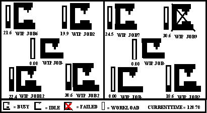
Figure 4: State of system objects during simulation
The extensive easy-to-use capabilities of the object-oriented system make the creation, storing, and updating of diagrams in the graphic interface quite straightforward. Pop-up menus and windows combined with the use of the mouse increase the speed of use of the system and minimize errors.
2. The second class is the Textual User Interface (TUI). This class depicts all class objects that represent a different interface from that presented in the GUI. When at the beginning of the process, the user selects the option of running the system without animation, the system automatically switches to the textual interface phase (non-graphic mode), where the computer internally processes all operations. In this phase, nothing is shown on the screen until the end of phase three is reached or the user interrupts to view a particular result. Execution time in this phase is faster than obtained from the graphic phase. The end of the execution or an interruption by the user is immediately followed by automatic display of a list of menu items which allows the user to select options for viewing the set for condensed results of the entire system, the individual cell, the machine or the job.
3. The third and final phase of user interaction involves the presentation and interpretation of the final result. The final result built under the class DisplayRules is displayed in a tabular form, with options to display information on all or a selected class object.
System Design Overview
The following describes how the object classes are grouped to functional areas within the object-oriented program.
1. System Function: The primary tasks of this group of classes are to create, modify, and store utilities, symbols and data used for processing in the system. These also define or report on the external entities and data stored.
2. Model Definition: The Model definition group includes all those modules whose major tasks are to define the statement of the problem and create the model that is used to solve the defined problem.
3. System Execution: The task of this group of classes is executing the process in part or in totality. A driver module is built-in which when invoked will execute methods according to the desired choice of the user.
4. System Report: The task of the system report group is to display the contents of data dictionaries (when required) in a given format. These also present the analysis result obtained at the end of the execution mode.
Management and Utilization of The Simulation System
In this system, a simulation continues to evolve as long as new data become available. Although objects such as demands, parts, processPlan and machinecell exist independently, they communicate with each other through the message-passing utility inherent within the environment. This allows dynamic responses to change during scheduling periods and the use of schedule improvement or tuning techniques. During execution, an initial schedule is developed based on the process plan, demand and machine requirements. After all of the required jobs have been scheduled, schedule evaluations are carried out to determine the next action to be taken by the simulation system. If the schedule developed is found to be feasible and optimal, the simulation process is terminated and the results presented. Otherwise, the System Improvement module is called upon to fine-tune the schedule.
Any system object can be in one of two possible states (active or inactive) at a given time. A part object is active when any of its operations are being processed and is inactive when it is not on any machine. An object can be down due to reasons which include machine failure or blocking. Activity times are established within the system. These include processing times, as well as breakdown and repair times. The setup and unloading times are assumed to be included in the processing times, and inspection times are considered as part of the activity of resources.
Scheduling Policies
In this scheduling system, either a static reactive or a dynamic scheduling policy can be adopted. The static reactive policy deals with an environment where at time zero, the decision maker establishes a list specifying the order in which the jobs will be processed and a list of relevant variables. The order of processing in a full static policy once established at time zero is not allowed to change. However, for static reactive scheduling, the order established at time zero is constantly revisited to reflect the current state of the system. Static reactivity redefines the system elements to correspond with any changes that may occur by allowing other jobs to arrive into the system. These arriving jobs are treated with the same importance as all the other jobs already scheduled.
Dynamic policy deals with an environment in which elements of the system remain unpredictable. As in static reactive scheduling, several jobs can be available at the beginning of the scheduling horizon, and these jobs are all scheduled a priori after which jobs continue to arrive into the system. As a result of the dynamic environment, scheduling modifications need to be made on existing elements to accommodate any changes. For example, machines break down sporadically, and when this happens, the effect on the system needs to be immediately evaluated and necessary action taken.
For the recent research using this simulation system, an exponential distribution was used for both job arrivals into the system and machine breakdown. Machine repair rate followed an Erlang distribution. Each machine had its own breakdown and repair rate. Job arrival rates differ according to the individual part in the job. Further details of the research are given in Olumolade and Norrie20, 21.
Rescheduling conditions
Rescheduling of jobs will occur in this system according to the following criteria:
a) Machine failure describes the non-availability of a broken-down machine.
b) A FixedTime condition depends on a management decision. It describes a fixed time during the simulation when a rescheduling can be performed.
c) Jobswaiting complements the fixed time. A rescheduling is performed when the number of jobs waiting to be scheduled is equal or greater than a given fixed number of jobs.
d) System empty defines a time during the simulation when neither of the above conditions (a or b) is true and all machines have completed all assigned operations and are idle.
If any of the above occur, rescheduling can result in modified due dates. A feasibility check is also carried out to determine the status of all the jobs in the system. In this check, all jobs (except for Work-In-Process (WIP)), have their completion times compared with their secondary due date. The secondary due date is the date after which the customer will not accept the job even if completed. The primary due date is the date after which the job, if not completed begins to incur penalties. All jobs that are not completed before or on the secondary due date are removed from the system for management reassessment.
The rescheduling feasibility check also includes jobs that, due to their inability to satisfy any of the earlier schedulability (materials, tools and system status or capability) criteria, have been considered unschedulable in a previous check and are still being held in the system because they satisfy the due date criterion. This process reduces the rescheduling time as it minimizes the number of jobs waiting to be rescheduled. In addition, it provides an opportunity for negotiation with customers if and when the reason for non-reschedulability of a job is due-date related.
Experimental Run
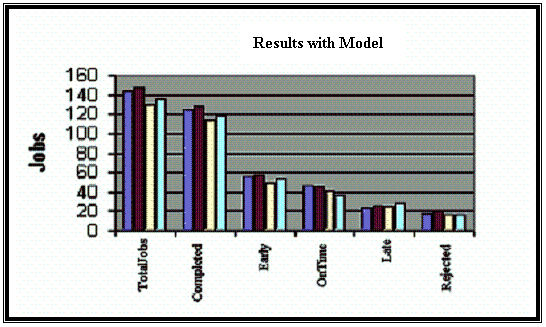
The system was tested under two different scenarios; first without implementing the model thus described and then with the model. In each case, the system started with four different jobs with each job having associated with it a size of 48, a due date, and process plan. After an initial feasible schedule of all these existing jobs, the simulation was enacted with jobs coming in at an exponential rate. During each run, three machine failures were introduced. The result is shown in the bar graph Figures 5a and b, the system with the model shows an overall improvement of 29%
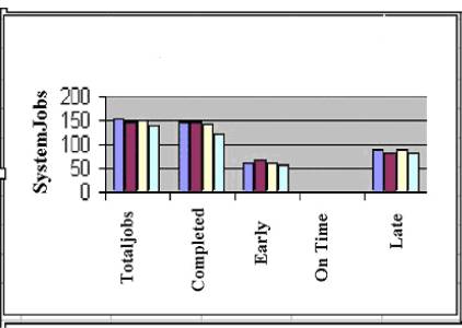
Figure 5a: Implementation without using the model
|
|
Figure 5b: Implementation with model
Summary
An object-oriented simulation model was developed for testing and evaluating an intelligent manufacturing scheduling system. The object-oriented architecture allowed a modular structure to be implemented, with real-life object mapping and flexibility with regard to subsequent changes. The scheduling system which was modeled incorporates both static and dynamic scheduling policies. In the latter case, the system is reactive with respect to machine failure and the affected jobs are dynamically rescheduled if the expected repair time exceeds a specified idle time. The simulation system showed the advantages of the object-oriented approach for embedded event-schedulers within a larger, more complex system.
References
1. Bispo, C. F. G. and J. J. Sentienro (1988), “An extended horizon scheduling algorithm for the job-shop problem.” IEEE Transactions, 17(2) 827 – 842.
2. Boukachour, J (1992), “Job shop simulation based on Object-oriented programming.” Proceedings of the society of computer simulation 1992 Western simulation multiconference on Object-oriented simulation. Beaumariage T. G. and R. K. Ege (editors) 8 – 12.
3. Broker, J, and K. Kosber (1992), “Improved communication system design using Object-oriented techniques.” Proceedings of the society of computer simulation 1992 Western simulation multiconference on Object-oriented simulation. Beaumariage T. G. and R. K Ege (editors) 3 – 7.
4. Chen, D., Luh, P. B., Thakur, L. S., and Moreno Jr. J. (2003), “Optimization-based manufacturing scheduling with multiple resources, setup requirements and transfer lots.” IIE Transactions, 35(10), 973 – 985.
5. Chryssolorous, G., and Subramaniam, V. (2001) “Dynamic scheduling of manufacturing job shop using Genetic Algorithm.” Journal of Intelligent Manufacturing, 12(3), 281 – 293.
6. Denton, B. and Gupta, D. (2003) “A sequential bounding approach for optimal appointment scheduling.” IIE Transaction, 35(11), 1003 – 1016.
7. Donath, M. and R. J. Graves (1998) “Flexible assembly systems: An application for near real-time scheduling and routing of multiple products.” International journal of production research, 26(12) 1903 – 1919.
8. Feuer, Z., R. Givon, and E. Dar‑El (1989), "A Simulation‑Based Scheduling System." The FMS Magazine, 7(1), pp. 15 ‑ 17.
9. Hardgrave, B. C. and Johnson, R. (2003), “Toward an Information system development acceptance model: The case of Object-oriented system development.” IEEE Transactions on engineering Management, 50(3), 322 – 336.
10. Jans, R. and Degrave, Z. (2004), “An Industrial extension of the discrete lot-size and scheduling problem.” IIE Transactions, 56(1), 47 – 58.
11. Keung, C. W., IP, W. H., and Lee, T. C. (2001), “Genetic algorithm approach to the multiple machine tool selection problems.” Journal of Intelligent Manufacturing, 12(1) 331 – 342.
12. Kurz, M. E. and Askin, R. G. (2003), “Comparing scheduling rules for flexible flow lines.” International journal of production economics, 85(3) 371 – 388.
13. Kurz, M. E. and Askin, R. G. (2001), “Heuristic scheduling of parallel machines with sequence-dependent set-up times.” International Journal of Production Research, 39(16) 3747-3769
14. Laporte, G., Salazar-Gonzalez, J. J. and Semet, F (2004), “Exact algorithm for job sequencing and lot switching problem.” IIE Transactions, 36(1) 37 – 45.
15. Law, A. M. and Kelton, W. D. (2000), “Simulation Modeling and Analysis.” 3rd edition, McGraw-Hill Boston, MA.
16. Mandelbaum, M. and Hlynka, M. (2003), “Job sequencing using an expert.” International journal of production economics, 85(3) 389 – 401.
17. Melnyk, S. A., S. Ghosh, and G. L. Ragatz (1989), “Tooling constraints and shop floor scheduling: A simulation study.” Journal of operations management, 8(2) 69 – 89.
18. Melouk, S., Damodaran, P. and Chang, P. (2004), “Minimizing makespan for single machine batch processing with non-identical job sizes using simulated annealing.” International journal of production economics, 87(2) 141 – 147.
19. Morton, D. P. and Popola, E. (2004), “A Bayesian stochastic programming approach to the employee scheduling problem.” IIE Transactions, 36(2) 155 – 167.
20. Olumolade, M., and Norrie, D. H. (1993), “Real Time Control of Manufacturing Scheduling Systems.” Proceedings of the IASTED International Conference on Applied Modeling and Simulation, Vancouver, Canada, July 21-23. 127 – 131.
21. Olumolade, M., and Norrie, D. H. (1996), “Reactive scheduling system for cellular manufacturing with failure-prone machines.” International Journal of Computer Integrated Manufacturing, 9(2) 131 – 144.
22. Phojanamongkolkij, N, Grabentetter, N. and Ghrayeb, O. (2003), “Scheduling jobs to improve weighted on-time performance of a single machine.” Journal of manufacturing systems, 22(2) 148 – 156.
23. Radhakrishnan, S. and Ventura, J. A. (2000), “Simulated annealing for parallel machine scheduling with earliness tardiness penalties and sequence dependent set-up times.” International Journal of Production Research, 38(10) 2233 – 2252.
24. Son, Y., Joshi, S. B., Wysk, R. A., and Smith, J. S. (2002), “Simulation-Based Shop Floor Control.” Journal of manufacturing systems, 21(5) 380 – 394.
25. Son, Y., Wysk, R. A. and Jones, A. T. (2003), “Simulation based shop floor control: Formal model, mode generation, and control interface.” IIE Transaction on Design and manufacturing, (35(1) 29 – 48.
26. Thomasma, T., Y. Mao, and O. M. Ulgen (1990), “Defining behavior in a hierarchical Object-oriented simulation program generator.” Proceedings of the summer simulation conference. Calgary, Canada. 266 – 271.
27. Young, H. L., Bhaskaran, K. and Pinedo, M. (1997), “A heuristic to minimize the total weighted tardiness with sequence-dependent setups.” IIE Transactions, 29(1) 45 – 52.
28. Zhang, G., Cai, X. and Wong, C. K. (2004), “Some results on resource constrained scheduling.” IIE Transactions, 36(2) 1 – 9.
29. Zobel, R. N. and A. M. Cummings (1990), “Experience in the development and use of an Object-oriented simulation environment for digital signal processing.” Proceedings of the summer computer simulation conference, Calgary, Canada. 867 – 873.