Volume 1, Number 1, Fall 2000

The use of simulation software with Monte Carlo techniques makes engineering economy problem solutions more realistic. Probability descriptions of input variables and Monte Carlo sampling together provide a practical method of finding the distribution of the desired output given the various random and deterministic input variables. The results of such analyses give better information for making decisions.

This paper provides solutions to three engineering economy problems. It shows that commonly available simulation software can be used to solve these problems. The first solution determines the future worth distribution of an annual series of payments when there is uncertainty about the future earning power from year to year. The second solution models the uncertainty of interest rates and the uncertainty of project life in order to generate the net present value distribution of a project. Finally, the third solution uses simulation to compare alternative investment opportunities under uncertainty.

Some information required for an engineering economic problem can be well defined, like the cost of new machinery, labor rates or the current tax rate structure. Much required information is uncertain, such as the actual cash flows from revenues and costs, the salvage value of equipment, the interest rate or even the project life. In most undergraduate engineering economy courses, the concept of risk is either not introduced at all or is mentioned briefly at the end of a course and in final chapters of a textbook⁷. Yet, engineering economy problems with all deterministic inputs are actually rare in "real life."

There are a number of approaches for handling economic risk that are used today. One approach is scenario analysis. However, as Park has pointed out, worst-case and best-case scenarios are not easy to interpret and do not provide probabilities of occurrence of those possibilities nor do they normally provide additional information such as the probability of losing money on a project or the probability of other possibilities¹². Sensitivity analysis and spider plots can provide insight into a engineering economy problems but are not appropriate when there is statistical dependence between variables⁵. Probability descriptions of input variables allow further refinement of the analysis of economic risk and allow the output of a distribution for the desired answer.

The notion of probability distributions to describe economic risk has been around for many years before the advent of computers and advanced software technology. Hillier, in his groundbreaking paper in 1963, proposed the use of probability distributions of present worth to properly convey project risk information to augment other methods such as expected value of the present worth and sensitivity analysis of individual inputs⁸. He also demonstrated that the probability distribution of present worth, or annual worth or internal rate of return can under certain assumptions be derived from yearly cash flows that are themselves random variables. He presented equations for the net present worth (NPV) distribution parameters when the cash flows were mutually independent random variables and when the cash flows were random but perfectly correlated to each other. Later, Giaccotto derived the distribution parameters for the NPV when the cash flows were correlated by a first order autoregressive stochastic process (or a Markov process).⁶ As projects become complicated, derivations of the probability distribution of the NPV as a function of the unknown random input variables can be tedious or impossible¹⁴.

Monte Carlo sampling provides a practical method of finding the distribution of the NPV or future worth from the various random input variables. Coats and Chesser showed that Monte Carlo techniques could be used in the corporate financial model to produce associated probabilities of occurrence, confidence intervals and standard deviations in addition to standard financial reports⁴. Seila and Banks showed that an electronic spreadsheet could be used to simulate project risk with Monte Carlo techniques¹⁴. The methods for risk analysis of projects have been published for a long time and the availability of computers and software is pervasive. Ho and Pike report that "proponents of risk analysis argue that increased risk information improves management’s understanding of the nature of risks, helps identify the major threats to project profitability and reduces forecasting errors⁹." They also report that "the risk analysis approach provides useful insights into the project, improves decision quality and increases decision confidence."⁹ But, the risk analysis approach is one aspect of economic analyses that is commonly ignored during project evaluations. Typically, deterministic data is "forced" even when there is uncertainty. The values are usually random, but are made to be point estimates without regard to the risk or sensitivity of error induced by assuming point estimates. Therefore, the outcome of the analysis has a greater probability of being wrong. A good project could be rejected or a bad project approved erroneously. Including risk analyses in engineering economy solutions is an important step to achieving more accurate information to make better decisions. Simulation with Monte Carlo techniques is one way to do risk analysis in engineering economy solutions.

Below is a chart that illustrates the differences between Hillier’s approach and a simulation approach for solving engineering economy problems.

Risk analysis approaches are covered in a few college class curriculums, but never fully to the extent that is necessary for graduates to be competent in industry. Risk analysis has been typically ignored not just because of the lack of knowledge but also because in the past it was cumbersome and difficult to implement or use. It was very time consuming and any software available was very expensive and needed large computers systems. Then, with the advent of personal computers (PC), spreadsheet capabilities, cheaper simulation software, and ease of use, performing risk analysis is easy. Numbers can be "crunched" and many simulation replications can be done in a small amount of time on relatively inexpensive computers.

Given that the capabilities of doing risk analyses are available, Goyal et al. has questioned why there is so little exposure to the stochastic nature of project cash flows and other project variables in undergraduate curricula⁷. Many in industry know that risk analyses exist, but few can apply the concepts to practice.

Computer simulation packages, using Monte Carlo techniques, are readily available and are particularly well suited for sampling from various theoretical and data-defined statistical distributions. In addition, these simulation packages can handle large amounts of sampling data and they have good output reporting capabilities. The next sections will demonstrate the ease that engineering economy problems with stochastic input variables can be simulated with industrial simulation software. Two different simulation software packages were used for the solutions. Arena was used for the first problem and SLAM II was used for the second and third problem.

One typical class of engineering economy problems involves calculating the future worth of a series of cash flows. As an example, suppose that we want to save $10,000 per year for the next 10 years. We would naturally be interested in how much worth would be accumulated at the end. If the growth rate was fixed and known, then the calculation of the future worth would be straightforward. However, it is important to note that in the real world there are many investment possibilities where the growth rate is variable from year to year. So, in this problem, the annual growth rate is the only variable that is uncertain. The other inputs are the $10,000 cash series and the 10 year project life. Both are deterministic data.

Suppose that the investment vehicle chosen was an S&P 500 index fund. The annual returns from 1954 till 1993 given by Bernstein indicate that the arithmetic average annual return was 13.1% and the overall equivalent annual return over the entire 40 years was 11.75%¹. However, the individual annual returns can vary from –26.5% to 52.6 %. This variability of annual returns and their timing of the more extreme values can create substantially different final results. The standard future worth formula ignores this variability and can only give a point estimate. Using simulation with Monte Carlo techniques to sample the annual return distribution to generate the multiple possible outcomes would better represent the actual economic situation.

The random returns of this problem were determined to be independent by first plotting the returns as shown in Figure 1. Then the correlation values of the different time lags of the annual returns were plotted as shown in Figure 2. Figure 2 shows that the annual returns are essentially independent from year to year.

Fig. 1. Time Plot of Annual Returns for the S&P 500 Index

Fig. 2. Correlation of Annual Returns over Time

Next, a simulation software package, Arena was used to determine the distribution of the data. Arena can either use historical data directly in the simulation or it can automate the process of fitting a probability distribution to the data. If a probability distribution is fitted to the data, Arena allows the user to select an appropriate distribution or Arena can select the closest fitting distribution itself¹⁰. For the S&P 500 annual returns, Arena chose the normal distribution with a mean of 13.1% and a standard deviation of 16.9% as the best fitting distribution. Unless there was a theoretical reason that called for a particular distribution, a good approach is to allow Arena to choose the best-fit distribution. The Arena choice of the normal distribution as best fit agrees with Bernstein¹. The fit is shown in Figure 3. Because the annual returns are independent and normally distributed, this simplifies the problem of generating random variables for the simulation.

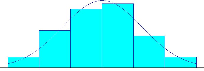
Fig. 3 Fit of Normal Curve to Historical S&P 500 Index Annual Returns

Finally, the simulation software was used to estimate the future worth distribution of this problem with the following steps:

• Each entity in the simulation run represents a replication (scenario) of the future worth calculation.
• After an entity is created, the annual growth rates (interest rates) are selected via sampling from the selected distributions.
• The sampled data is attached to the entity as attributes.
• The future worth associated with the entity is calculated and stored as another attribute.
• Before the entity leaves the system, the future worth is collected as a statistic and tabulated by the simulation software.

There are several methods for stopping the simulation. For this problem, the method chosen was to limit the number of created entities to 5000, which gave 5000 replications. The Arena network diagram to simulate this problem is given in Figure 4.

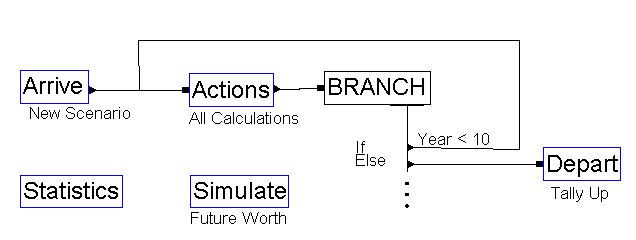
Fig.4. Simulation Network Diagram For Future Worth Estimation with Variable Interest Rates

The output of the simulation program is given in Figure 5. Because each entity was created one time unit apart, the current time on the Arena report also reflects the number of replications in the study (5000). The output reporting capabilities of simulation packages are used to advantage here. Summary statistics are automatically generated. It shows that the future worth of the 5000 scenarios ranges from $61,366 to $397,660. Any prediction (tolerance) interval can be determined using the histogram. For example, it appears that 90% of the observations fall between $90,000 to $230,000. This means there is a 90% confidence that the future worth of this series falls between $90,000 and $230,000. From the text output, the mean expected value is $154,280. Incidentally, if we had used the standard equal payment series future worth calculation with 10 years at 11.75% fixed annual return, the point estimate would have been $173,380 with no indication of the probable range.

                            ARENA Simulation Results
                 Dr. Eyler Robert Coates, Jr. - License #9910153

                        Summary for Replication 1 of 1

Project:  Future Worth                        Run execution date :  12/ 4/1999
Analyst:  Endt and Coates                     Model revision date:  12/ 4/1999

Replication ended at time      : 5000.0

                                 TALLY VARIABLES

Identifier              Average   Half Width  Minimum    Maximum   Observations
_______________________________________________________________________________

Future Amount           1.5428E+05 1175.7     61366.     3.9766E+05   5000    

                                   COUNTERS

                    Identifier                Count   Limit
                    _________________________________________

                    Replications               5000  Infinite


Simulation run time: 0.08 minutes.
Simulation run complete.

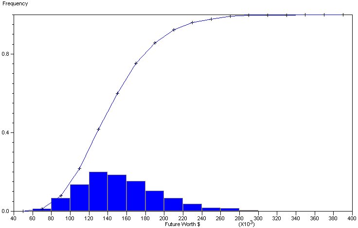
Fig. 5. Simulation Output from Network in Fig. 4

Hillier presented equations for the net present worth (NPV) distribution parameters when the cash flows were mutually independent random variables Using Hillier’s original example as a basis for problem 2, Table 1 gives the mutually independent normally distributed cash flows from Hillier's problem⁸.

Table 1. Estimated Net Cash Flow Data

Hillier has shown that the resultant net present value (NPV) is also normally distributed with the parameters given by Equations 1 and 2. Assume that the interest rate, i, is 10%.

However, by adding complications to the problem makes closed form equations for the NPV difficult or impossible to derive. Suppose that the interest rate can vary from year to year and the project life is uncertain. Then, it would be more practical to use simulation to estimate the NPV distribution.

As in Problem 1, simulation software such as SLAM II or Arena (SLAM II was used for this problem) could be used to estimate the NPV distribution by the following steps:

• Each entity in the simulation run represents a replication (scenario) of the NPV calculation.
• After an entity is created, input data is selected via sampling from distributions.
• The sampled data is attached to the entity as attributes.
• The NPV associated with the entity is calculated and stored as another attribute.
• Before the entity leaves the system, the NPV is collected as a statistic and tabulated by the simulation software.

For this example, the expected values of each year’s cash flows are stored in an array as follows: ARRAY(1,1) = -400, ARRAY(1,2) = 120, …, ARRAY(1,6) = 200. The standard deviations are also stored in an array as follows: ARRAY(2,1) = 20, ARRAY(2,2) = 10, …, ARRAY(2,6) = 50.

In this model, the interest rate is allowed to take on an initial random starting value (with mean of 10% and a standard deviation of 0.5%) and each subsequent year’s rate is generated by a first order autoregressive stochastic process. In this example, the correlation of interest rates from one year to the next is 80% and the noise component is normally-distributed with 0 mean and 1% standard deviation. From Giaccotto⁶, this type of autoregressive series can be modeled by

The project life span itself is also allowed to vary from 4 to 6 years with a 25% chance that the project will last 4 years, a 50% chance that the project will last 5 years and a 25% chance that the project will last 6 years. It takes little effort to build the simulation network to accommodate variability in yearly cash flows, interest rates over the life of the project and variability in the project life span itself. This is evident by the elegant structure of the network in Fig. 6. The array of cash flow parameters is expanded by the addition of ARRAY(1,7) = 200 and ARRAY(2,7) = 50 to accommodate the new possibility of cash flow in the 6^th year of the project. The output of the simulation program with variable cash flows, interest rates and project life span as simulated in Fig. 6 is given in Fig. 7.

Fig. 6. Network Diagram For NPV Problem With Variable Cash Flows, Interest Rate and Project Life

                S L A M   I I   S U M M A R Y   R E P O R T

  SIMULATION PROJECT SIMPLE ECONOMIC RISK      BY EYLER COATES        
  DATE  2/12/1998                              RUN NUMBER    1 OF    1

  CURRENT TIME   0.5000E+04
  STATISTICAL ARRAYS CLEARED AT TIME  0.0000E+00

            **STATISTICS FOR VARIABLES BASED ON OBSERVATION**
                   MEAN    STANDARD  COEFF. OF  MINIMUM   MAXIMUM  NO.OF
                   VALUE   DEVIATION VARIATION   VALUE      VALUE    OBS

 PRESENT VALUE   0.935E+02 0.987E+02 0.106E+01 -.154E+03 0.394E+03  5000

Fig. 7. Simulation Output from Network in Fig. 6

Coates has already indicated the importance of including the variability of interest rates and project life when appropriate³. He noted that the probability of a negative NPV went from 2.3% in Hillier’s original problem to 20.9% when the additional variability of the interest rate and the project life was included. The mean NPV for both problems was essentially unchanged, but the standard deviation of the NPV distribution had doubled. Thus, using expected values only and ignoring variability of input data has its perils.

The comparison of alternative systems is one of the most important uses of simulation². In this case of engineering economy problems, the alternative systems often take the form of alternative projects. Furthermore, these projects are often mutually exclusive. That is, the decision maker can choose only one of the alternative projects to invest in. Therefore, an analysis of the alternatives can be conducted to select the best investment. As discussed earlier, as the projects become more complex, simulation provides a convenient and powerful means of conducting such an analysis.

The following example illustrates the use of simulation to compare the investments of two alternative projects based on their net present value. For simplicity, we will let the first alternative be a fixed 5 year project having the same interest rate and cash flow distributions described in Problem 2 where the net expected cash flows for each period are described in Table 1. The second alternative also has the same characteristics with the exception of the net expected cash flows that are shown in Table 2.

A common method used for comparing alternatives is to compare the difference in the expected net present values for the two investments. To do this, a confidence interval can be constructed on the difference between population means. Therefore, we can construct a simulation model for each alternative as before and obtain independent observations of the net present value for each project. However, since we are using simulation to obtain these observations, variance reduction techniques such as common random numbers can be used to improve the quality of our estimate¹¹. With the introduction of common random numbers, the corresponding independent observations of the net present value from each project will be treated as matched pairs when constructing the confidence interval.

The network diagram of the simulation model that incorporates common random numbers is shown in Figure 8. Here, as before, the mean and standard deviation of the yearly cash flows are stored in a two dimensional array. Statistics are collected on the net present value of each alternative. In addition, the 5000 independent observations of NPV are written to the output file "NPV.DAT". These data are then read into a spreadsheet program to construct the confidence interval. (Note that some simulation packages, like Arena, could provide more elaborate output analysis tools that enable you to conduct this type of analysis).

Table 2. Estimated Net Cash Flow Data for Alternative 2.

Fig. 8. Network Diagram For Problem 3.

A point estimate of the mean difference in net present value between Alternative 2 and Alternative 1, respectively is 65.59 and a 95% confidence interval of the mean difference is

From this confidence interval we can conclude that on average investing in Alternative 2 will yield a significantly higher return than Alternative 1. However, in most investment problems, the decision maker will only have one opportunity to invest in any particular project. Therefore, perhaps a more appropriate analysis tool would be to construct a tolerance interval (or prediction interval) on the difference in NPV for a single investment. That is, one can construct a tolerance interval such that the probability that a single observation will fall within the interval is at least some specified quantity¹³. For this example, a 95% tolerance interval on the difference in net present value on a single investment is

This tolerance interval indicates that a single investment in either Alternative 1 or Alternative 2 may yield a higher return over the other investment opportunity. Consequently, this method of analysis provides information to the decision maker on one-time only investments that is often overlooked.

As the alternatives under consideration become more complex in terms of the uncertainty involved in cash flow characteristics, interest rates, etc. simulation provides a means of analyzing problems when closed form analytical solutions do not exist.

The three problem solutions presented in this paper demonstrate how commonly available simulation software could be used in engineering economy problems. The first problem solution generated the future worth distribution of an annual series of payments when there is uncertainty about the future earning power (interest rate) from year to year. The second problem solution simulated the uncertainty of interest rates and the uncertainty of project life in order to generate the NPV distribution of a project. Finally, the last problem solution showed that simulation software can be used effectively for the comparison of alternative investments under uncertainty. These problem solutions can be used as examples to demonstrate how risk can be handled in an engineering economy course. They can also be used as additional applications in an industrial simulation course.

1. Bernstein, P.L., [1995], The Portable MBA in Investment, John Wiley and Sons, New York, NY.
2. Banks, J., J.S. Carson II, B.L. Nelson, [1996], Discrete-Event System Simulation, Second Edition, Prentice Hall, New Jersey.
3. Coates, E.R., [1999], Project Risk Simulation Using Off-The-Shelf Simulation Software, Proceedings of the 25^th International Conference on Computers and Industrial Engineering - New Orleans, LA, March 1999, 457-460.
4. Coats, P.K., and D.L. Chesser, [1982], Coping With Business Risk Through Probabilistic Financial Statements, Simulation, June 1982, 111-121.
5. Eschenbach, T.G., and R.J. Gimpel, [1990], Stochastic Sensitivity Analysis, The Engineering Economist, 35(4), 305-321.
6. Giaccotto, C., [1984], A Simplified Approach To Risk Analysis In Capital Budgeting With Serially Correlated Cash Flows, The Engineering Economist, 29(4), 273-286.
7. Goyal, A.K., J.M. Tien, and P.A. Voss, [1997], Integrating Uncertainty Considerations In Learning Engineering Economy, The Engineering Economist, 42(3), 249-257.
8. Hillier, F.S., [1963], The Derivation of Probabilistic Information For The Evaluation Of Risky Investments, Management Science, 1963, 443-457.
9. Ho, S.S.M., and R.H. Pike, [1998], Organizational Characteristics Influencing The Use Of Risk Analysis In Strategic Capital Investments, The Engineering Economist, 43(3), 247-268.
10. Kelton, W.D., R.P. Sadowski, and D.A. Sadowski, [1998], Simulation with Arena, WCB/McGraw-Hill, Boston, MA.
11. Law, A.M. and W.D. Kelton, [1991], Simulation Modeling and Analysis, Second Edition, McGraw-Hill, Inc., New York.
12. Park, C.S., [1997], Contemporary Engineering Economics, 2^nd Edition, Addison-Wesley, Menlo Park CA.
13. Pritsker, A.A.B., [1995], Introduction to Simulation and SLAM II, 4^th Edition, John Wiley and Sons, New York.
14. Seila, A.F., and J. Banks, [1990], Spreadsheet Risk Analysis Using Simulation, Simulation, 57, 163-170.