Volume 1, Number 2, Spring 2001

---

A Combined Stress Experiment Using a Hacksaw

 

Marshall F. Coyle
Pennsylvania State University-York
1031 Edgecomb Ave.
York, PA 17403-3398
Email: mfc5@psu 

Christal G. Keel
Pennsylvania State University-York
Email: christal@keel.org 

 

ABSTRACT

This paper describes a laboratory experiment that can be used to demonstrate combined stresses to engineering students in Strength of Materials classes. A typical hand-held hacksaw is used to illustrate combined normal stresses due to bending and axial loading. A commercially available handsaw is loaded statically by tension in the saw blade. The tensile load on the hacksaw blade results in both bending and axial compressive stresses in the backbone of the hacksaw. This study demonstrates the experimental technique of using strain gages to validate an analytical solution, as well as the concept of creating and calibrating a load transducer to measure the applied load. This paper presents details on the analysis, experimental approach, and the results.

INTRODUCTION

The purpose of the experiment is to demonstrate a basic concept of combine stresses that engineering students typically encounter in their first Strength of Materials class. C-clamps, coping saws, and hacksaws are popular examples of combine stress problems presented in textbooks^{1, 2}. This paper differs from other laboratory experiments^{3, 4} using C-clamps in that its goal is to demonstrate the validation of an analytical approach. This not only helps to further students’ understanding of combined stress but also demonstrates the experimental validation portion of the design circle.

Figure 1 illustrates a typically constructed hand-held hacksaw.

 

 

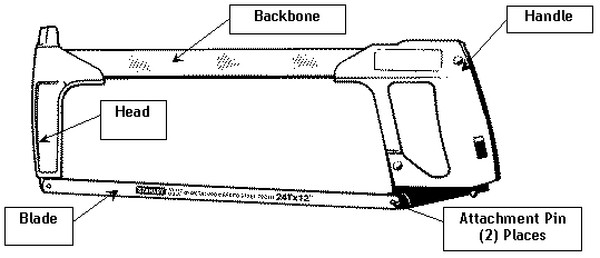
Figure 1: Typical Hacksaw.

 

The head, handle, and backbone make up the frame of the hacksaw. The rigidity of the frame places the blade in tension in order to prevent buckling due to the slenderness of the blade. When a tensile force is applied to the blade, the head and handle portions of the saw see a resulting tension. These forces produce both axial compressive forces and bending forces in the backbone of the saw. A Stanley contractor grade high-tension saw was chosen for this experiment, due to the following characteristics:

• It has a quick blade tightener/release mechanism that facilitates a rapid and easily repeatable loading and unloading of the blade.
• The blade tension is adjustable up to 340 lb.
• The backbone consists of rectangular, chrome-plated steel tubing that allows for the effective application of strain gages.
• The distance between the centerline of the saw blade and the backbone varies linearly, with the smaller distance occurring at the head. This causes the bending moment to vary along the length of the saw and makes for a more interesting analysis.

 

THEORY

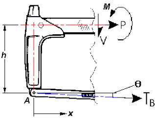
Figure 2: Free body diagram of saw head and backbone.

Figure 2 is a Free Body Diagram (FBD) of an arbitrary section taken through the saw. The shear force (V), bending moment (M), and axial force (P) are all shown as being in the positive direction for the standard beam convention. The blade is a two-force member that produces a point load applied at point A. Since the blade sits in the frame at a slight angle (q), the resultant force will have X and Y components. The tensile force in the blade (T_B) is counteracted by both an axial compressive force (P) and a shear force (V) in the backbone. This axial compressive force serves to balance the horizontal component of the tensile force (T_B) while the shear force (V) balances the vertical component.

 

SF_x = 0                                                                                                            (1)

P + T_B * cos(q) = 0

P = -T_B * cos(q)

SF_y = 0                                                                                                            (2)

                        -V - T_B  * sin(q) = 0

V = -T_B  * sin(q)

 

Because both the horizontal and vertical components of T_B being applied at point A are eccentric to the axis of the backbone a bending moment (M) is produced. It is calculated as follows:

 

SM_A = 0                                                                                     (3)

M – P * h – V * x = 0

                        M = P * h + V * x

                        M = -T_B * cos(q) * h – T_B * sin(q) * x

 

where h is the vertical distance from point A to the neutral axis of the backbone and x is the horizontal distance from point A to the location of the section. Figure 3 shows the cross-section of the backbone. The axial stress (s_A) in the backbone is calculated by dividing the resultant compressive force (P) by the cross sectional area of the backbone (A):

 

s_A = P/ A                                                                                                         (4)

 

 

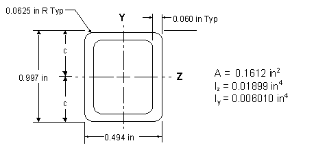
Figure 3: Cross-sectional drawing of the backbone.

 

The bending moment produces a bending stress (s_B), which is tensile on the top and compressive on the bottom surfaces of the saw’s backbone. We can now use the flexure formula to calculate the bending stresses:

 

            s_B = ± M * c / I_z                                                                                                                         (5)

 

where c is the distance from the neutral axis to the outer surfaces of the backbone as illustrated in Figure 3, and I_Z is the moment of inertia about the Z-axis.

The strains on the top (e _top) and the bottom (e _bottom) of the backbone are calculated by dividing the combined stresses by the modulus of elasticity (E = 29.0E6 psi for steel):

 

            e _top = (s_B-top + s_A) / E                                                                                     (6)

            e _bottom = (s_B-bottom + s_A) / E                                                                              (7)

 

EXPERIMENTAL VERIFICATION

I. Instrumentation:

The Stanley High-Tension Hacksaw was instrumented with eight Measurements Group, Inc. EA-06-240LZ-120 Student Gages. The strain gage locations are shown in Figure 4 and listed in Table 1.

 

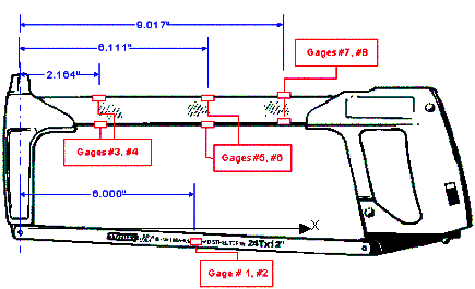
Figure 4: Mounting locations of strain gages

 

Table 1: Gage Locations

The backbone is instrumented with six strain gages, three along the top surface, and three along the bottom surface of the backbone. Two strain gages are also located on the saw blade, since it is used as a load transducer. The strain gages on the saw blade were placed back-to-back on the front and backsides of the saw blade in order to average out any effects due to bending in the saw blade. The gages were bonded to the hacksaw with a Measurements Group, Inc. M-Bond 200 cyanoacrylate adhesive system. Strain gage readings were taken using Measurements Group, Inc. P-3500 Portable Strain Indicator with a SB-10 Switch and Balance Unit.

II. Load Transducer Calibration:

Calibration of the load transducer was accomplished by acquiring strain gage readings for various tensile loads. The instrumented saw blade was placed in a test frame shown in Figure 5 and instrumented with a 0-5,000 kg dynamometer. The transducer was loaded from 0 to 551 lb in 55.1 lb increments, and strain gage readings were taken at each increment. A linear regression analysis was performed on the calibration data. Figure 6 presents the results from the load transducer calibration showing a plot of the load versus strain. It can be seen from the plot that the behavior of the load transducer is linear.

 

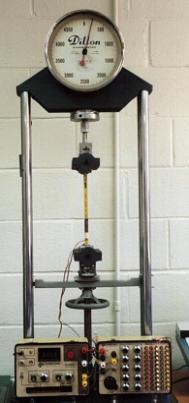
Figure 5: Photograph of test frame set-up.

 

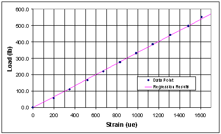
Figure 6: Load Transducer Behavior.

III. Experimental Procedure:

The saw blade (load transducer) was positioned on the hacksaw attachment pins, which were located on the head and handle of the saw as illustrated in Figure 1. The strain gage balance unit was used to zero all the strain gage readings. Tension was then applied to the saw blade by using the saw’s tensioning mechanism. The strain gage readings from the loaded hacksaw were recorded, at which point the tension was removed from the blade. Strain gage readings were taken after the load was removed to determine instrumentation drift, which was found to be a maximum of 6 µe. This test procedure was replicated four times.

DISCUSSION OF RESULTS

There was good agreement between the experimental and the analytical results for all four experimental replications. The applied load varied from 304.5 to 306.7 lb among the replications, which produced slightly different analytical and experimental results. The difference between the analytical and experimental results was consistent between the four replications. It varied less than 0.90 % for each location between replications; therefore, only the results from one replication are presented. The analytical and experimental results from one of the experiments are tabulated in Table 2 and graphically shown in Figure 7.

Table 2: Analytical and Experimental Results 

 

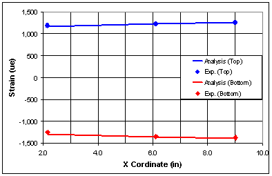
Figure 7: Analytical and Experimental Results

The results presented in Table 2 and Figure 7 come from a test having a test load (T_B) of 305.5 lb. Results show there is good agreement between the analytical and experimental results. The greatest difference was –2.41 %, which occurred at gage #4. The difference between the analytical and experimental results is due to gage location measurements that were taken. Errors in measurement h shown in Figure 2 will affect the analytical solution the most.

SUMMARY

A simple hand-held hacksaw that most people are probably familiar with was used to demonstrate the concepts of axial, bending, and combined stresses and strains. This paper outlined an analytical procedure for calculating the stresses and strains in the backbone of a conventional hacksaw. The analytical results were then verified experimentally. This paper gives details on the experimental procedure using strain gages to validate the analytical solution. Finally, analytical and experimental results are presented showing that there is good agreement between the two.

REFERENCES

1.      Applied Strength of Materials, 3rd edition, by Robert L. Mott, MacMillan Publishing, pp. 421-422, 1996. ISBN 0-13-376278-5.

2.      Mechanics of Materials, 4th edition, by R.C. Hibbeler, Prentice Hall, pp. 434-437, 2000. ISBN 0-13-016467-4.

3.      Of Clamps & Spring & Things: http://www.measurementsgroup.com/guide/notebook/e22/e22.htm, Measurements Group, Inc., last accessed April 17, 2001.

4.      A Strength of Materials Laboratory Experiment: http://et.nmsu.edu/~etti/spring98/mechanical/magill/magill.html, Michael A. Magill, Ph.D., P.E., last accessed April 17, 2001.